Features and Options
Dimensional analysis
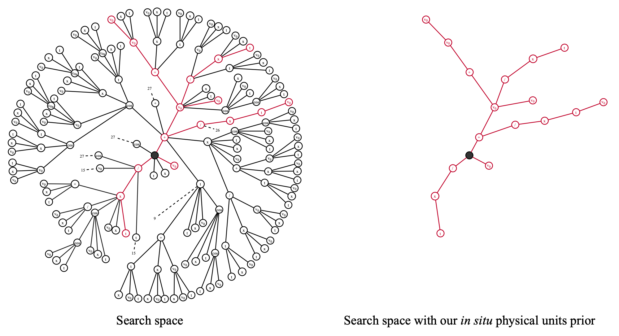
physo provides a physical units feature that can be used to reduce the symbolic expression search space by enforcing dimensional analysis constraints.
Reference paper for this feature: [Tenachi 2023].
This feature can simply be used by passing the units of the variables and root through X_units and y_units arguments, as well as units of constants through fixed_consts_units and free_constants_units (and if necessary through spe_free_consts_units and class_free_consts_units for Class SR).
In addition, PhysicalUnitsPrior should be enabled in the priors_config list of the run configuration, this is the case for all available configurations in the physo/config/ directory.
See the getting-started-sr tutorial where this feature is used.
Exploiting multiple datasets
physo can exploit multiple datasets by searching for a single analytical functional form that accurately fits multiple datasets - each governed by its own (possibly) unique set of fitting parameters.
We dub this framework (introduced in [Tenachi 2024]) “Class Symbolic Regression” (Class SR).
See the Class SR documentation.
Priors
About Priors
We provide a number of priors that can be used to guide the symbolic regression process and reduce the search space by tuning the probability of selecting certain symbols during the generation of the candidate expressions.
For using a prior, a tuple should be added to the priors_config list in the run configuration (see physo/config/ for examples of configurations).
The first element of the tuple should be the name of the prior class, and the second element should be the parameters to be passed to the prior.
These should parametrize the prior class as required in their __init__ method (except for library, program args which are handled by the algorithm itself).
List of priors
Uniform Arity Prior
- class physo.physym.prior.UniformArityPrior(library, programs)
Uniform probability distribution over tokens by their arities. This prior encourages tokens with an arity that is under-represented and discourages tokens with an arity that is over-represented by normalising token probabilities by the number of tokens having its arity.
- __init__(library, programs)
- Parameters:
library (library.Library) –
programs (vect_programs.VectPrograms) –
Example of usage from the config file:
priors_config  = [
                ...
                ("UniformArityPrior", None),
                ...
                 ]
Hard Length Prior
- class physo.physym.prior.HardLengthPrior(library, programs, min_length, max_length)
Forces programs to have lengths such that min_length <= lengths <= max_length finished. Enforces lengths <= max_length by forbidding non-terminal tokens when choosing non-terminal tokens would mean exceeding max length of program. Enforces min_length <= lengths by forbidding terminal tokens when choosing a terminal token would mean finishing a program before min_length.
Example of usage from the config file:
priors_config  = [
                ...
                ("HardLengthPrior"  , {"min_length": 4, "max_length": 35, }),
                ...
                 ]
Soft Length Prior
- class physo.physym.prior.SoftLengthPrior(library, programs, length_loc, scale)
Soft prior that encourages programs to have a length close to length_loc. Before loc: scales terminal token probabilities by gaussian where dangling == 1 (ie. programs that might finish next step). After loc: scales non-terminal token probabilities by gaussian.
Example of usage from the config file:
priors_config  = [
                ...
                ("SoftLengthPrior"  , {"length_loc": 8, "scale": 5, }),
                ...
                 ]
Relationship Constraint Prior
- class physo.physym.prior.RelationshipConstraintPrior(library, programs, effectors, relationship, targets, max_nb_violations=None)
Forces programs to comply with relationships constraints. Enforcing that [targets] cannot be the [relationship] of [effectors]. Where targets are choosable tokens for the current batch, effectors are already chosen tokens having a [relationship] relationship (descendant, child or sibling) with targets. This constraint between elements of effectors list and targets list in a one to one fashion so effectors and targets list should have the same size. Eg. effectors = [“sin”, “n2”, “exp”], relationship = “child”, targets = [“cos”, “sqrt”, “log”] forbids cos from being the child of sin, sqrt from being the child of n2 and log from being the child of exp.
- __init__(library, programs, effectors, relationship, targets, max_nb_violations=None)
Enforcing that [targets] cannot be the [relationship] of [effectors]. :param library: :type library: library.Library :param programs: :type programs: vect_programs.VectPrograms :param effectors: List of effector tokens’ name. :type effectors: list of str :param relationship: Relationship to forbid between effectors and targets (“descendant”, “child” or “sibling”). :type relationship: str :param targets: List of target tokens’ name. :type targets: list of str :param max_nb_violations: List containing max number of acceptable violations for each constraint relationship in case there are
multiple relatives having [relationship] with [targets] (eg. multiple ancestors). By default = None, zero violations are allowed. Should have the same size as effectors and targets lists. Remark: using max_nb_violations with values > 0 on single relative relationship cases (eg. parent) would mean applying no constraint whatsoever.
Example of usage from the config file:
priors_config  = [
                ...
                ("RelationshipConstraintPrior"  , {"effectors"    : ["exp" , "log", "sin", "exp", "sub"],
                                                   "targets"      : ["log" , "exp", "sin", "cos", "neg"],
                                                   "relationship" : "child",
                                                   }),
                ...
                 ]
No Useless Inverse Prior
- class physo.physym.prior.NoUselessInversePrior(library, programs)
Forbids useless inverse sequences. Enforcing that op can not be the child of op^(-1) and that op^(-1) can not be the child of op for all op having an inverse op^(-1) listed in functions.INVERSE_OP_DICT.
- __init__(library, programs)
Enforcing functions are not child of their inverse function. :param library: :type library: library.Library :param programs: :type programs: vect_programs.VectPrograms
Example of usage from the config file:
priors_config  = [
                ...
                ("NoUselessInversePrior"  , None),
                ...
                 ]
Nested Functions
- class physo.physym.prior.NestedFunctions(library, programs, functions, max_nesting=1)
Regulates nesting for a group of tokens. Enforcing that any token in [functions] can only have up to [max_nesting] ancestors listed in [functions].
- __init__(library, programs, functions, max_nesting=1)
Enforcing that [functions] can not be nested or only up to max_nesting level. :param library: :type library: library.Library :param programs: :type programs: vect_programs.VectPrograms :param functions: List of tokens’ names which’s nesting will be forbidden. :type functions: list of str :param max_nesting: Max level of nesting allowed. By default = 1, no nesting allowed. :type max_nesting: int
Example of usage from the config file:
priors_config  = [
                ...
                ("NestedFunctions", {"functions":["exp",], "max_nesting" : 1}),
                ("NestedFunctions", {"functions":["log",], "max_nesting" : 1}),
                ...
                 ]
Nested Trigonometry Prior
- class physo.physym.prior.NestedTrigonometryPrior(library, programs, max_nesting=1)
Regulates nesting of trigonometric functions listed in functions.TRIGONOMETRIC_OP. Enforcing that any trigonometric function can only have up to [max_nesting] ancestors that also are trigonometric functions.
- __init__(library, programs, max_nesting=1)
Enforcing that trigonometric functions can not be nested or only up to max_nesting level. :param library: :type library: library.Library :param programs: :type programs: vect_programs.VectPrograms :param max_nesting: Max level of nesting allowed. By default = 1, no nesting allowed. :type max_nesting: int
Example of usage from the config file:
priors_config  = [
                ...
                ("NestedTrigonometryPrior", {"max_nesting" : 1}),
                ...
                 ]
Occurrences Prior
- class physo.physym.prior.OccurrencesPrior(library, programs, targets, max)
Enforces that [targets] can not appear more than [max] times in programs.
- __init__(library, programs, targets, max)
Example of usage from the config file:
priors_config  = [
                ...
                ("OccurrencesPrior", {"targets" : ["1",], "max" : [3,] }),
                ...
                 ]
Symbolic Prior
- class physo.physym.prior.SymbolicPrior(library, programs, expression)
Enforces that programs must be exactly like [expression].
- __init__(library, programs, expression)
- Parameters:
Example of usage from the config file:
priors_config  = [
                ...
                # Forcing expression to look like a + ...
                ('SymbolicPrior', {'expression': ["+", "a", ]}),
                ...
                 ]
Physical Units Prior
- class physo.physym.prior.PhysicalUnitsPrior(library, programs, prob_eps=0.0)
Enforces that next token should be physically consistent units-wise with current program based on current units constraints computed live (during program generation). If there is no way get a constraint all tokens are allowed.
Example of usage from the config file:
priors_config  = [
                ...
                # Zeroing out to epsilon level unphysical symbolic choices
                ("PhysicalUnitsPrior", {"prob_eps": np.finfo(np.float32).eps}),
                ...
                 ]
Weighting Data Points / Uncertainty Quantification in SR
About weights
physo provides a feature that allows the user to weight data points when performing symbolic regression.
This feature can be used to give more importance to certain data points over others - in order to take into account uncertainties in the data, or to favor certain parts of the dataset over others.
The weights are used during free constant optimization as well as for computing the reward driving the symbolic regression process.
Weights can simply be passed through the y_weights argument of physo.SR, they should have the same shape as the target values y.
Class SR notes:
If you are using Class SR, the weights should be passed through the multi_y_weights argument of physo.ClassSR.
They can have the same shape as the target values multi_y or simply the length of the number of realizations (for giving more weights to certain realizations over others), as indicated in the docstring of physo.ClassSR for more details).
Example
Example of weight usage in SR. The reference notebook for this tutorial can be found here: demo_y_weights.ipynb.
Setup
Importing the necessary libraries:
# External packages
import numpy as np
import matplotlib.pyplot as plt
import torch
Importing physo:
# Internal code import
import physo
import physo.learn.monitoring as monitoring
It is recommended to fix the seed for reproducibility:
# Seed
seed = 0
np.random.seed(seed)
torch.manual_seed(seed)
Making synthetic datasets
Making a toy synthetic dataset:
# Making toy synthetic data
t = np.random.uniform(0.1, 10, 1000)
X = np.stack((t,), axis=0)
y = np.exp(-1.45*t) + 0.5*np.cos(3.7*t)
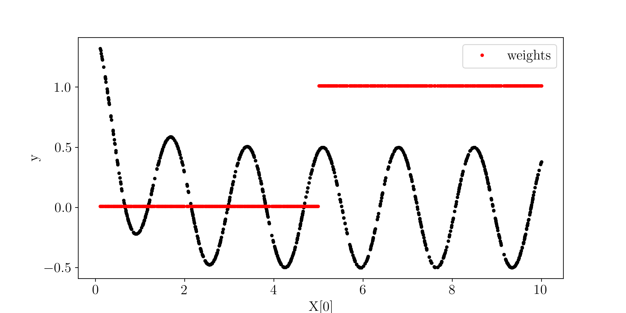
Let’s give more weight to the latter part of the dataset which should favor the cosine term:
y_weights = 0.01 + (t > 5.).astype(float)
Datasets plot:
n_dim = X.shape[0]
fig, ax = plt.subplots(n_dim, 1, figsize=(10,5))
for i in range (n_dim):
    curr_ax = ax if n_dim==1 else ax[i]
    curr_ax.plot(X[i], y, 'k.',)
    curr_ax.set_xlabel("X[%i]"%(i))
    curr_ax.set_ylabel("y")
    # Weights
    curr_ax.plot(X[i], y_weights, 'r.', label="weights")
    curr_ax.legend()
plt.show()
SR configuration
Logging and visualisation setup:
save_path_training_curves = 'demo_curves.png'
save_path_log             = 'demo.log'

run_logger     = lambda : monitoring.RunLogger(save_path = save_path_log,
                                                do_save = True)

run_visualiser = lambda : monitoring.RunVisualiser (epoch_refresh_rate = 1,
                                           save_path = save_path_training_curves,
                                           do_show   = False,
                                           do_prints = True,
                                           do_save   = True, )
Running SR
# Running SR task
expression, logs = physo.SR(X, y,
                            y_weights = y_weights,
                            # Giving names of variables (for display purposes)
                            X_names = [ "t"   ],
                            # Giving name of root variable (for display purposes)
                            y_name  = "y",
                            # Fixed constants
                            fixed_consts       = [ 1.      ],
                            # Free constants names (for display purposes)
                            free_consts_names = [ "c1", "c2", "c3",],
                            # Symbolic operations that can be used to make f
                            op_names = ["mul", "add", "sub", "div", "inv", "n2", "sqrt", "neg", "exp", "log", "sin", "cos"],
                            get_run_logger     = run_logger,
                            get_run_visualiser = run_visualiser,
                            # Run config
                            run_config = physo.config.config0.config0,
                            # Parallel mode (only available when running from python scripts, not notebooks)
                            parallel_mode = False,
                            # Number of iterations
                            epochs = 30
)
Inspecting the best expression found
Getting best expression:
The best expression found (in accuracy) is returned in the expression variable:
best_expr = expression
print(best_expr.get_infix_pretty())
>>>
       ⎛     c₃⋅c₃⋅(c₂ + c₂ + c₃ + c₃ + t)⎞
    sin⎜c₂ + ─────────────────────────────⎟
       ⎝                  1.0             ⎠
    ───────────────────────────────────────
                       c₃
It can also be loaded later on from log files:
import physo
from physo.benchmark.utils import symbolic_utils as su
import sympy

# Loading pareto front expressions
pareto_expressions = physo.read_pareto_pkl("demo_curves_pareto.pkl")
# Most accurate expression is the last in the Pareto front:
best_expr = pareto_expressions[-1]
print(best_expr.get_infix_pretty())
Checking exact symbolic recovery
# To sympy
best_expr = best_expr.get_infix_sympy(evaluate_consts=True)

best_expr = best_expr[0]

# Printing best expression simplified and with rounded constants
print("best_expr : ", su.clean_sympy_expr(best_expr, round_decimal = 4))

# Target expression was:
target_expr = sympy.parse_expr("0.5*cos(3.7*t)")
print("target_expr : ", su.clean_sympy_expr(target_expr, round_decimal = 4))

# Check equivalence
print("\nChecking equivalence:")
is_equivalent, log = su.compare_expression(
                        trial_expr  = best_expr,
                        target_expr = target_expr,
                        round_decimal = 1,
                        handle_trigo            = True,
                        prevent_zero_frac       = True,
                        prevent_inf_equivalence = True,
                        verbose                 = True,
)
print("Is equivalent:", is_equivalent)
>>> best_expr :  0.5194*sin(3.7062*t + 26.6575)
    target_expr :  0.5*cos(3.7*t)

    Checking equivalence:
      -> Assessing if 0.5*cos(3.7*t) (target) is equivalent to 0.519443317596468*sin(3.70615580351008*t + 26.6574530128894) (trial)
       -> Simplified expression : 0.5*sin(3.7*t + 26.7)
       -> Symbolic error        : -0.5*sin(3.7*t + 26.7) + 0.5*cos(3.7*t)
       -> Symbolic fraction     : cos(3.7*t)/sin(3.7*t + 26.7)
       -> Trigo symbolic error        : 0
       -> Trigo symbolic fraction     : 1
       -> Equivalent : True
    Is equivalent: True
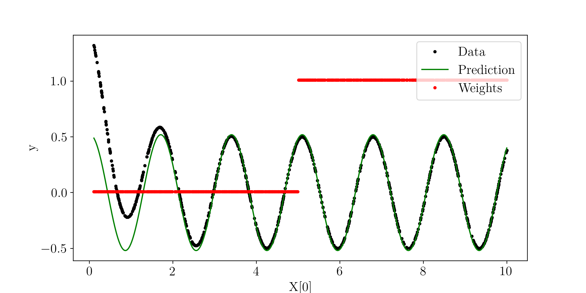
Fit plot
# Reloading expression
best_expr = pareto_expressions[-1]
# Making predictions
X_extended = np.stack( [np.linspace(X.min(), X.max(), 1000),] )
y_pred = best_expr(torch.tensor(X_extended))
Plot:
n_dim = X.shape[0]
fig, ax = plt.subplots(n_dim, 1, figsize=(10,5))
for i in range (n_dim):
    curr_ax = ax if n_dim==1 else ax[i]
    # Data
    curr_ax.plot(X[i], y, 'k.', label="Data")
    # Prediction
    curr_ax.plot(X_extended[i], y_pred, 'g-', label="Prediction")
    # Weights
    curr_ax.plot(X[i], y_weights, 'r.', label="Weights")
    curr_ax.legend(loc="upper right")
    # Labels
    curr_ax.set_xlabel("X[%i]"%(i))
    curr_ax.set_ylabel("y")
plt.show()
Candidate wrapper
The candidate_wrapper argument can be passed to the physo.SR or physo.ClassSR to apply a wrapper function \(g\) to the candidate symbolic function’s output \(f(X)\).
The wrapper function \(g\) should be a callable taking the candidate symbolic function callable \(f\) and the input data \(X\) as arguments, and returning the wrapped output \(g(f(X))\).
By default candidate_wrapper = None, no wrapper is applied (identity).
Note that the wrapper function should be differentiable and written in pytorch if free constants are to be optimized since the free constants are optimized using gradient-based optimization.
In addition, it is recommended to use protected functions when writing the wrapper function to avoid evaluating the symbolic function on invalid points (eg. using log abs instead of log). See the protected functions documentation for more details.
Adding custom functions
Defining function token
If you want to add a custom choosable function to physo, you can do so by adding you own Token to the list OPS_UNPROTECTED in functions.py.
For example a token such as \(f(x) = x^5\) can be added via:
OPS_UNPROTECTED = [
...
Token (name = "n5"     , sympy_repr = "n5"     , arity = 1 , complexity = 1 , var_type = 0, function = lambda x :torch.pow(x, 5)         ),
...
]
Where:
name(str) is the name of the token (used for selecting it in the config of a run).sympy_repr(str) is the name of the token to use when producing the sympy / latex representation.arity(int) is the number of arguments that the function takes.complexity(float) is the value to consider for expression complexity considerations (1 by default).var_type(int) is the type of token, it should always be 0 when defining functions like here.function(callable) is the function, it should be written in pytorch to support auto-differentiation.
More details about Token attributes can be found in the documentation of the Token object : here
Behavior in dimensional analysis
The newly added custom function should also be listed in its corresponding behavior (in the context of dimensional analysis) in the list of behaviors in OP_UNIT_BEHAVIORS_DICT (here).
Additional information
In addition, the custom function should be :
Listed in
TRIGONOMETRIC_OP(here) if it is a trigonometric operation (eg. cos, sinh, arcos etc.) so it can be treated as such by priors if necessary.Listed in
INVERSE_OP_DICT(here) along with its corresponding inverse operation \(f^{-1}\) if it has one (eg. arcos for cos) so they can be treated as such by priors if necessary.Listed in
OP_POWER_VALUE_DICT(here) along with its power value (float) if it is a power token (eg. 0.5 for sqrt) so it can be used in dimensional analysis.
Protected version (optional)
If your custom function has a protected version ie. a version defined everywhere on \(\mathbb{R}\) (eg. using \(f(x) = log(abs(x))\) instead of \(f(x) = log(x)\) ) to smooth expression search and avoid undefined rewards, you should also add the protected version in to the list OPS_PROTECTED in functions.py with the similar attributes but with the protected version of the function for the function attribute.
Running the functions unit test (optional)
After adding a new function, running the functions unit test is highly recommended:
python ./physo/physym/tests/functions_UnitTest.py
If you found the function you have added useful, don’t hesitate to make a pull request so other people can use it too !