Benchmarks
This section presents the benchmarking utilities available within physo : user-friendly ways to access benchmarking challenges in a reproducible and standardized manner (using standard data ranges etc.).
For each challenge, we present ways to generate data and compare candidate expressions to the ground truth.
Our interfaces adhere to the standard benchmarking practices presented in [La Cava 2021].
Feynman benchmark
The purpose of the Feynman benchmark is to evaluate symbolic regression systems, in particular methods built for scientific discovery. That is methods able to produce compact, predictive and interpretable expressions from potentially noisy data.
See [Udrescu 2019] which introduced the benchmark, [La Cava 2021] which formalized it and [Tenachi 2023] for the evaluation of physo on this benchmark.
Note that physo reads Feynman challenges from the original files (FeynmanEquations.csv, BonusEquations.csv, units.csv) produced by [Udrescu 2019] and adjusting for some mistakes (incorrect units, columns etc.) in the original files.
Loading a Feynman challenge
This benchmark comprises 120 challenges, each with a unique ground truth expression.
Challenge number i_eq \(\in\) {0, 1, …, 119} of the Feynman benchmark ({0, …, 99} corresponding to bulk challenges and {100, …, 119} to bonus challenges) can be accessed as follows:
import physo
import physo.benchmark.FeynmanDataset.FeynmanProblem as Feyn

i_eq = 42
pb = Feyn.FeynmanProblem(i_eq=i_eq)
print(pb)
>>> FeynmanProblem : I.42 : I.42
    x0*exp((-x1)*x2*x4/((x3*x5)))
It is also possible to access the problem with its original variable names:
print(Feyn.FeynmanProblem(i_eq, original_var_names=True))
>>> FeynmanProblem : I.40.1 : I.40.1
    n_0*exp(g*(-m)*x/((T*kb)))
Getting formula and variable infos
Getting sympy formula, also encodes assumptions on variables (positivity, etc.):
print(pb.formula_sympy)
>>> x0*exp((-x1)*x2*x4/((x3*x5)))
Getting latex formula:
print(pb.formula_latex)
>>> 'x_{0} e^{\\frac{- x_{1} x_{2} x_{4}}{x_{3} x_{5}}}'
Getting names of variables and their units:
print(pb.X_names)
>>> array(['x0', 'x1', 'x2', 'x3', 'x4', 'x5'], dtype='<U2')
print(pb.X_units)
>>> array([[ 0.,  0.,  0.,  0.,  0.],
           [ 0.,  0.,  1.,  0.,  0.],
           [ 1.,  0.,  0.,  0.,  0.],
           [ 0.,  0.,  0.,  1.,  0.],
           [ 1., -2.,  0.,  0.,  0.],
           [ 2., -2.,  1., -1.,  0.]])
print(pb.y_name)
>>> 'y'
print(pb.y_units)
>>> array([0., 0., 0., 0., 0.])
Generating data
Generating 1000 data points:
X, y = pb.generate_data_points(n_samples=1000)
print(X.shape) # (n_variables, n_samples)
>>> (6, 1000)
print(y.shape) # (n_samples,)
>>> (1000,)
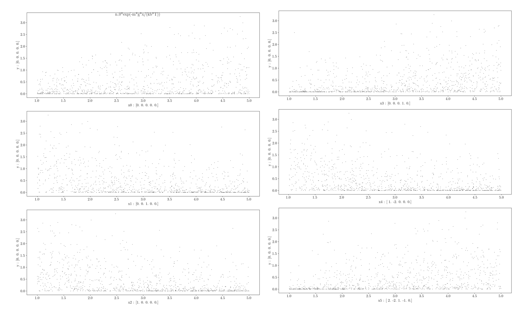
Showing 1000 data points:
pb.show_sample(1000)
Target function
It is possible to evaluate the target function using:
y = pb.target_function(X)
Assessing symbolic equivalence of a candidate expression
Given a candidate expression, we can assess its symbolic equivalence to the ground truth expression.
# Expression returned by SR system:
candidate_expr_str = "1.0002*x0*exp(0.0004-x1*x2*0.9993*x4)**(1/(x3*x5))+0.00034"
Getting a sympy expression from the string:
import sympy
candidate_expr = sympy.parse_expr(candidate_expr_str,
                                 # Encoding assumptions about variables (positivity etc.)
                                 local_dict = pb.sympy_X_symbols_dict)
Comparing it to the ground truth (using [La Cava 2021] standard methodology):
is_equivalent, report = pb.compare_expression(trial_expr    = candidate_expr,
                                              round_decimal = 3,
                                              verbose       = True
                                             )
>>>
      -> Assessing if x0*exp(-x1*x2*x4/(x3*x5)) (target) is equivalent to 1.0002*x0*(1.00040008001067*exp(-0.9993*x1*x2*x4))**(1/(x3*x5)) + 0.00034 (trial)
       -> Simplified expression : x0*exp(-x1*x2*x4/(x3*x5))
       -> Symbolic error        : 0
       -> Symbolic fraction     : 1
       -> Trigo symbolic error        : 0
       -> Trigo symbolic fraction     : 1
       -> Equivalent : True
Class benchmark
The purpose of the Class benchmark is to evaluate Class symbolic regression systems, that is: methods for automatically finding a single analytical functional form that accurately fits multiple datasets - each governed by its own (possibly) unique set of fitting parameters.
See [Tenachi 2024] in which we introduce this first benchmark for Class SR methods and evaluate physo on it.
Loading a Class challenge
This benchmark comprises 8 challenges, each with a unique ground truth expression but a range of possible values for dataset-specific free constants (K).
Challenge number i_eq \(\in\) {0, 1, …, 7} of the Class benchmark can be accessed as follows:
import physo
import physo.benchmark.ClassDataset.ClassProblem as ClPb

i_eq = 4
pb = ClPb.ClassProblem(i_eq=i_eq)
print(pb)
>>> ClassProblem : 4 : Damped Harmonic Oscillator B
    exp(-0.345*x0)*cos(k0*x0 + k1)
It is also possible to access the problem with its original variable names:
print(ClPb.ClassProblem(i_eq, original_var_names=True))
>>> ClassProblem : 4 : Damped Harmonic Oscillator B
    exp(-0.345*t)*cos(Phi + omega*t)
Getting formula and variable infos
Getting sympy formula, also encodes assumptions on variables (positivity, etc.):
print(pb.formula_sympy)
>>> exp(-0.345*x0)*cos(k0*x0 + k1)
Getting latex formula:
print(pb.formula_latex)
>>> e^{- 0.345 x_{0}} \cos{\left(k_{0} x_{0} + k_{1} \right)}
Getting names of variables:
print(pb.X_names)
>>> ['x0']
print(pb.y_name)
>>> 'y'
Getting names of dataset-specific free constants and their ranges:
print(pb.K_names)
>>> ['k0', 'k1']
print(pb.K_lows)
>>> [0.6 -0.2]
print(pb.K_highs)
>>> [1.4 0.3]
Generating data
Generating 1000 data points across 5 realizations:
multi_X, multi_y, K = pb.generate_data_points(n_samples=1000, n_realizations=5, return_K=True)
print(multi_X.shape) # (n_realizations, n_variables, n_samples)
>>> (5, 1, 1000)
print(multi_y.shape) # (n_realizations, n_samples)
>>> (5, 1000)

print(K.shape)
>>> (5, 2)
Showing 1000 data points across 10 realization:
pb.show_sample(n_samples=1000, n_realizations=10)

Target function
It is possible to evaluate the target function on a dataset realization X using its associated dataset-specific free constants K via:
y = pb.target_function(multi_X[0], K=[0.123, 0.456])
Assessing symbolic equivalence of a candidate expression
Let’s consider that a Class SR system has been run on a dataset having this ground truth expression (for say realization 0):
# Ground truth expression having dataset-specific free constant values [0.123, 0.456]:
target_expr = pb.get_sympy(K_vals=[[0.123, 0.456]])[0]
Let’s consider that the Class SR system has returned the following candidate expression for this realization 0:
# Expression returned by Class SR system on a dataset realization:
candidate_expr_str = "exp(-0.345004*x0)*sin(0.5*3.141592 - 0.123002*x0 - 0.456001) + 0.0043"
Getting a sympy expression from the string:
import sympy
candidate_expr = sympy.parse_expr(candidate_expr_str,
                                 # Encoding assumptions about variables (positivity etc.)
                                 local_dict = pb.sympy_X_symbols_dict)
Comparing it to the ground truth (using [La Cava 2021] standard methodology):
import physo.benchmark.utils.symbolic_utils as su

# Comparing on realization 0
is_equivalent, report = su.compare_expression(trial_expr   = candidate_expr,
                                              target_expr  = target_expr,
                                              round_decimal = 1,
                                              verbose       = True
                                             )
>>>
    -> Assessing if exp(-0.345*x0)*cos(0.123*x0 + 0.456) (target) is equivalent to 0.0043 - exp(-0.345004*x0)*sin(0.123002*x0 - 1.114795) (trial)
     -> Simplified expression : -exp(-0.3*x0)*sin(0.1*x0 - 1.1)
     -> Symbolic error        : (sin(0.1*x0 - 1.1) + cos(0.1*x0 + 0.5))*exp(-0.3*x0)
     -> Symbolic fraction     : -cos(0.1*x0 + 0.5)/sin(0.1*x0 - 1.1)
     -> Trigo symbolic error        : 0
     -> Trigo symbolic fraction     : 1
     -> Equivalent : True
Adding noise
Adding a noise fraction NOISE_LEVEL \(\in\) [0, 1] as in [La Cava 2021] to data:
import numpy as np

y_rms = ((y ** 2).mean()) ** 0.5
epsilon = NOISE_LEVEL * np.random.normal(0, y_rms, len(y))
y = y + epsilon