Class Symbolic Regression
About Class SR
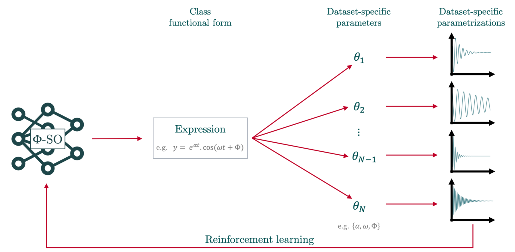
Class Symbolic Regression (Class SR) is a method for automatically finding a single analytical functional form that accurately fits multiple datasets - each governed by its own (possibly) unique set of fitting parameters. This hierarchical framework leverages the common constraint that all the members of a single class of physical phenomena follow a common governing law.
See [Tenachi 2024] in which we introduce Class SR.
Getting started (Class SR)
In this tutorial, we show how to use physo to perform Class Symbolic Regression (Class SR) by exploiting 4 datasets.
The reference notebook for this tutorial can be found here: class_sr_quick_start.ipynb.
Setup
Importing the necessary libraries:
# External packages
import numpy as np
import matplotlib.pyplot as plt
import torch
Importing physo:
# Internal code import
import physo
import physo.learn.monitoring as monitoring
It is recommended to fix the seed for reproducibility:
# Seed
seed = 0
np.random.seed(seed)
torch.manual_seed(seed)
Making synthetic datasets
Making toy synthetic datasets: here a simple 4 realizations linear problem where the numerical parameters governing the dependency on the x0 variable and the offset are different for each realization:
multi_X = []
multi_y = []

# Realization 0
x0 = np.random.uniform(-10, 10, 256)
x1 = np.random.uniform(-10, 10, 256)
X = np.stack((x0, x1), axis=0)
y = 1.123*x0 + 1.123*x1 + 10.123
multi_X.append(X)
multi_y.append(y)

# Realization 1
x0 = np.random.uniform(-11, 11, 500)
x1 = np.random.uniform(-11, 11, 500)
X = np.stack((x0, x1), axis=0)
y = 2*1.123*x0 + 1.123*x1 + 10.123
multi_X.append(X)
multi_y.append(y)

# Realization 2
x0 = np.random.uniform(-12, 12, 256)
x1 = np.random.uniform(-12, 12, 256)
X = np.stack((x0, x1), axis=0)
y = 1.123*x0 + 1.123*x1 + 0.5*10.123
multi_X.append(X)
multi_y.append(y)

# Realization 3
x0 = np.random.uniform(-13, 13, 256)
x1 = np.random.uniform(-13, 13, 256)
X = np.stack((x0, x1), axis=0)
y = 0.5*1.123*x0 + 1.123*x1 + 2*10.123
multi_X.append(X)
multi_y.append(y)
Where multi_X and multi_y are lists containing \(n_{reals}\) realizations (here \(n_{reals}=4\)). multi_X should contain \(n_{reals}\) elements consisting of input variables values (\(X\)) (one per realization) and multi_y should contain \(n_{reals}\) corresponding target values (\(y\)) (one per realization).
Elements \(X\), \(y\) should respectively be of shape \((n_{dim}, ?,)\) and \((?,)\) where \(n_{dim}\) is the number of input variables (here \(n_{dim}=2\) as there are 2 input variables: \((x_0, x_1)\)) and ? is the number of data points (this number must be consistent across each \((X, y)\) pair but can depend on the realization).
It should be noted that free constants search starts around 1. by default. Therefore, when using default hyperparameters, normalizing the data around an order of magnitude of 1 is strongly recommended.
Datasets plot:
n_reals = len(multi_X)
fig, ax = plt.subplots(n_reals, 2, figsize=(12,20))

for i in range(n_reals):
    ax[i][0].plot(multi_X[i][0], multi_y[i], 'k.')
    ax[i][0].set_xlabel("x0")
    ax[i][0].set_ylabel("y (Realization %i)"%(i))
    ax[i][1].plot(multi_X[i][1], multi_y[i], 'k.')
    ax[i][1].set_xlabel("x1")
Class SR configuration
It should be noted that SR capabilities of physo are heavily dependent on hyperparameters, it is therefore recommended to tune hyperparameters to your own specific problem for doing science.
Summary of currently available hyperparameters presets configurations:
Config |
Recommended usecases |
Speed |
Effectiveness |
Notes |
|---|---|---|---|---|
|
Demos |
★★★ |
★ |
Light and fast config. |
|
SR with DA \(^*\) ; Class SR with DA \(^*\) |
★ |
★★★ |
Config used for Feynman Benchmark and MW streams Benchmark. |
|
SR ; Class SR |
★★ |
★★ |
Config used for Class Benchmark. |
\(^*\) DA = Dimensional Analysis
Users are encouraged to edit configurations (they can be found in: physo/config/).
By default, config0b is used, however it is recommended to follow the upper recommendations for doing science.
Class SR side notes:
It is recommended to always use the
bvariant (ie.configxb) of configurations for Class SR as these variants specify a larger number of steps for the free constants optimizations that is performed during expression candidate evaluation (this is necessary because all free constants specific to each realization are optimized at the same time which typically makes it necessary to have a larger number of optimization steps).Due to the typically higher number of free constants values to tune, Class SR is typically much more expansive computationally than regular SR, lower batch size configurations are therefore recommended.
DA side notes:
During the first tens of iterations, the neural network is typically still learning the rules of dimensional analysis, resulting in most candidates being discarded and not learned on, effectively resulting in a much smaller batch size (typically 10x smaller), thus making the evaluation process much less computationally expensive. It is therefore recommended to compensate this behavior by using a higher batch size configuration which helps provide the neural network sufficient learning information.
Logging and visualisation setup:
save_path_training_curves = 'demo_curves.png'
save_path_log             = 'demo.log'

run_logger     = lambda : monitoring.RunLogger(save_path = save_path_log,
                                                do_save = True)

run_visualiser = lambda : monitoring.RunVisualiser (epoch_refresh_rate = 1,
                                           save_path = save_path_training_curves,
                                           do_show   = False,
                                           do_prints = True,
                                           do_save   = True, )
Running Class SR
Automatically finding a single analytical functional form that accurately fits multiple datasets - each governed by its own (possibly) unique set of fitting parameters.
This hierarchical framework leverages the common constraint that all the members of a single class of physical phenomena follow a common governing law.
Ie. recovering a single analytical function \(f\) that best fits \(y_{i_{real}} = f_{i_{real}}(x_0, ..., x_{n_{dim}})\) for each realization \(i_{real} \leq n_{reals}\) of a phenomena given \({\{x_0, ..., x_{n_{dim}}\}}_{{i_{real}} \leq n_{reals}}\) (multi_X) data and \({\{y\}}_{{i_{real}} \leq n_{reals}}\) (multi_y) data.
Realization-specific free constants ie. free constants taking different values depending on the realization (\({\{k_0, k_1, ... \}}_{{i_{real}} \leq n_{reals}}\)) are designated as spe_free_consts and free constants common to the whole class (\(\{c_0, c_1, ... \}\)) are designated as class_free_consts.
# Running SR task
expression, logs = physo.ClassSR(multi_X, multi_y,
                            # Giving names of variables (for display purposes)
                            X_names = [ "x0"       , "x1"        ],
                            # Associated physical units (ignore or pass zeroes if irrelevant)
                            X_units = [ [0, 0, 0] , [0, 0, 0]    ],
                            # Giving name of root variable (for display purposes)
                            y_name  = "y",
                            y_units = [0, 0, 0],
                            # Fixed constants
                            fixed_consts       = [ 1.      ],
                            fixed_consts_units = [ [0, 0, 0] ],
                            # Whole class free constants
                            class_free_consts_names = [ "c0"      ,],
                            class_free_consts_units = [ [0, 0, 0] ,],
                            # Realization specific free constants
                            spe_free_consts_names = [ "k0"      , "k1"        ],
                            spe_free_consts_units = [ [0, 0, 0] , [0, 0, 0]   ],
                            # Run config
                            run_config = physo.config.config0b.config0b,
                            # Symbolic operations that can be used to make f
                            op_names = ["add", "sub", "mul", "div"],
                            get_run_logger     = run_logger,
                            get_run_visualiser = run_visualiser,
                            # Parallel mode (only available when running from python scripts, not notebooks)
                            parallel_mode = False,
                            # Number of iterations
                            epochs = 10,
)
Inspecting the best expression found
Getting best expression:
The best expression found (in accuracy) is returned in the expression variable:
best_expr = expression
print(best_expr.get_infix_pretty())
>>> c₀⋅(k₀ + k₁⋅(k₀⋅(k₁ + k₁) + k₀ + x₀) - k₁ + x₁ + x₁)
It can also be loaded later on from log files:
import physo
from physo.benchmark.utils import symbolic_utils as su
import sympy

# Loading pareto front expressions
pareto_expressions = physo.read_pareto_pkl("demo_curves_pareto.pkl")
# Most accurate expression is the last in the Pareto front:
best_expr = pareto_expressions[-1]
print(best_expr.get_infix_pretty())
Display:
The expression can be converted into…
A sympy expression:
best_expr.get_infix_sympy()
>>> 𝑐0(𝑘0+𝑘1(𝑘0(𝑘1+𝑘1)+𝑘0+𝑥0)−𝑘1+𝑥1+𝑥1)
A sympy expression (with evaluated free constants values):
# In Class SR this will return an array of expression each containing constants values specific to each realization:
best_expr.get_infix_sympy(evaluate_consts=True)
>>> array([1.12300062502826*x0 + 1.12299943170758*x1 + 10.1229929701024,
       2.24600237740662*x0 + 1.12299943170758*x1 + 10.1229940888655,
       1.12299855430429*x0 + 1.12299943170758*x1 + 5.0615011673083,
       0.561499701563431*x0 + 1.12299943170758*x1 + 20.2460066025792],
      dtype=object)
A latex string:
best_expr.get_infix_latex()
>>> 'c_\{0\} \\left(k_\{0\} + k_\{1\} \\cdot \\left(2 k_\{0\} k_\{1\} + k_\{0\} + x_\{0\}\\right) - k_\{1\} + 2 x_\{1\}\\right)'
A latex string (with evaluated free constants values):
sympy.latex(best_expr.get_infix_sympy(evaluate_consts=True))
>>> '\\mathtt\{\\text\{[1.12300062502826*x0 + 1.12299943170758*x1 + 10.1229929701024\n 2.24600237740662*x0 + 1.12299943170758*x1 + 10.1229940888655\n 1.12299855430429*x0 + 1.12299943170758*x1 + 5.0615011673083\n 0.561499701563431*x0 + 1.12299943170758*x1 + 20.2460066025792]\}\}'
Getting free constant values:
best_expr.free_consts
>>> FreeConstantsTable
     -> Class consts (['c0']) : (1, 1)
     -> Spe consts   (['k0' 'k1']) : (1, 2, 4)
Class free constants:
best_expr.free_consts.class_values
>>> tensor([[0.5615]], dtype=torch.float64)
Realization-specific free constants:
best_expr.free_consts.spe_values
>>> tensor([[[1.8208, 0.5954, 1.0013, 9.2643],
             [2.0000, 4.0000, 2.0000, 1.0000]]], dtype=torch.float64)
Checking exact symbolic recovery
# To sympy
best_expr = best_expr.get_infix_sympy(evaluate_consts=True)

best_expr = best_expr[0] # Considering the expression with its constants set for realization no 0 (Class SR)

# Printing best expression simplified and with rounded constants
print("best_expr : ", su.clean_sympy_expr(best_expr, round_decimal = 4))

# Target expression was:
target_expr = sympy.parse_expr("1.123*x0 + 1.123*x1 + 10.123")
print("target_expr : ", su.clean_sympy_expr(target_expr, round_decimal = 4))

# Check equivalence
print("\nChecking equivalence:")
is_equivalent, log = su.compare_expression(
                        trial_expr  = best_expr,
                        target_expr = target_expr,
                        handle_trigo            = True,
                        prevent_zero_frac       = True,
                        prevent_inf_equivalence = True,
                        verbose                 = True,
)
print("Is equivalent:", is_equivalent)
>>> best_expr :  1.123*x0 + 1.123*x1 + 10.123
    target_expr :  1.123*x0 + 1.123*x1 + 10.123

    Checking equivalence:
      -> Assessing if 1.123*x0 + 1.123*x1 + 10.123 (target) is equivalent to 1.12300062502826*x0 + 1.12299943170758*x1 + 10.1229929701024 (trial)
       -> Simplified expression : 1.12*x0 + 1.12*x1 + 10.12
       -> Symbolic error        : 0
       -> Symbolic fraction     : 1
       -> Trigo symbolic error        : 0
       -> Trigo symbolic fraction     : 1
       -> Equivalent : True
    Is equivalent: True
Function docstring
- physo.ClassSR(multi_X, multi_y, multi_y_weights=1.0, X_names=None, X_units=None, y_name=None, y_units=None, fixed_consts=None, fixed_consts_units=None, class_free_consts_names=None, class_free_consts_units=None, class_free_consts_init_val=None, spe_free_consts_names=None, spe_free_consts_units=None, spe_free_consts_init_val=None, op_names=None, use_protected_ops=True, stop_reward=1.0, max_n_evaluations=None, stop_after_n_epochs=10, epochs=None, candidate_wrapper=None, run_config=None, get_run_logger=None, get_run_visualiser=None, parallel_mode=True, n_cpus=None, device='cpu')
Runs a class symbolic regression task ie. searching for a single functional form fitting multiple datasets allowing each dataset to have its own realization specific free constant values (spe_free_consts) but using the same class free constants (class_free_consts) for all datasets. (Wrapper around physo.task.fit)
- Parameters:
multi_X (list of len (n_realizations,) of np.array of shape (n_dim, ?,) of float) – List of X (one per realization). With X being values of the input variables of the problem with n_dim = nb of input variables.
multi_y (list of len (n_realizations,) of np.array of shape (?,) of float) – List of y (one per realization). With y being values of the target symbolic function on input variables contained in X.
multi_y_weights (list of len (n_realizations,) of np.array of shape (?,) of float or array_like of (n_realizations,) of float or float, optional) – List of y_weights (one per realization). With y_weights being weights to apply to y data. Or list of weights one per entire realization. Or single float to apply to all (for default value = 1.).
X_names (array_like of shape (n_dim,) of str or None (optional)) – Names of input variables (for display purposes).
X_units (array_like of shape (n_dim, n_units) of float or None (optional)) – Units vector for each input variables (n_units <= 7). By default, assumes dimensionless.
y_name (str or None (optional)) – Name of the root variable (for display purposes).
y_units (array_like of shape (n_units) of float or None (optional)) – Units vector for the root variable (n_units <= 7). By default, assumes dimensionless.
fixed_consts (array_like of shape (?,) of float or None (optional)) – Values of choosable fixed constants. By default, no fixed constants are used.
fixed_consts_units (array_like of shape (?, n_units) of float or None (optional)) – Units vector for each fixed constant (n_units <= 7). By default, assumes dimensionless.
class_free_consts_names (array_like of shape (?,) of str or None (optional)) – Names of free constants (for display purposes).
class_free_consts_units (array_like of shape (?, n_units) of float or None (optional)) – Units vector for each free constant (n_units <= 7). By default, assumes dimensionless.
class_free_consts_init_val (dict of { str : float } or None (optional)) – Dictionary containing free constants names as keys (eg. ‘c0’, ‘c1’, ‘c2’) and corresponding float initial values to use during optimization process (eg. 1., 1., 1.). None will result in the usage of token.DEFAULT_FREE_CONST_INIT_VAL as initial values. None by default.
spe_free_consts_names (array_like of shape (?,) of str or None (optional)) – Names of free constants (for display purposes).
spe_free_consts_units (array_like of shape (?, n_units) of float or None (optional)) – Units vector for each free constant (n_units <= 7). By default, assumes dimensionless.
spe_free_consts_init_val (dict of { str : float } or dict of { str : array_like of shape (n_realizations,) of floats } or None, optional) – Dictionary containing realization specific free constants names as keys (eg. ‘k0’, ‘k1’, ‘k2’) and corresponding float initial values to use during optimization process (eg. 1., 1., 1.). Realization specific initial values can be used by providing a vector of shape (n_realizations,) for each constant in lieu of a single float per constant. None will result in the usage of token.DEFAULT_FREE_CONST_INIT_VAL as initial values. None by default.
op_names (array_like of shape (?) of str or None (optional)) – Names of choosable symbolic operations (see physo.physym.functions for a list of available operations). By default, uses operations listed in physo.task.args_handler.default_op_names.
use_protected_ops (bool (optional)) – If True, uses protected operations (e.g. division by zero is avoided). True by default. (see physo.physym.functions for a list of available protected operations).
stop_reward (float (optional)) – Early stops if stop_reward is reached by a program (= 1 by default), use stop_reward = (1-1e-5) when using free constants.
max_n_evaluations (int or None (optional)) – Maximum number of unique expression evaluations allowed (for benchmarking purposes). Immediately terminates the symbolic regression task if the limit is about to be reached. The parameter max_n_evaluations is distinct from batch_size * n_epochs because batch_size * n_epochs sets the number of expressions generated but a lot of these are not evaluated because they have inconsistent units.
stop_after_n_epochs (int or None (optional)) – Number of additional epochs to do after early stop condition is reached. Uses args_handler.default_stop_after_n_epochs by default.
epochs (int or None (optional)) – Number of epochs to perform. By default, uses the number in the default config file.
candidate_wrapper (callable or None (optional)) – Wrapper to apply to candidate program’s output, candidate_wrapper taking func, X as arguments where func is a candidate program callable (taking X as arg). By default = None, no wrapper is applied (identity).
run_config (dict or None (optional)) – Run configuration (by default uses physo.task.class_sr.default_config) See physo/config/ for examples of run configurations.
get_run_logger (callable returning physo.learn.monitoring.RunLogger or None (optional)) – Run logger (by default uses physo.task.args_handler.get_default_run_logger)
get_run_visualiser (callable returning physo.learn.monitoring.RunVisualiser or None (optional)) – Run visualiser (by default uses physo.task.args_handler.get_default_run_visualiser)
parallel_mode (bool (optional)) – Parallel execution if True, execution in a loop else. True by default. Overrides parameter in run_config.
n_cpus (int or None (optional)) – Number of CPUs to use when running in parallel mode. Uses max nb. of CPUs by default. Overrides parameter in run_config.
device (str (optional)) – Device to use for computations (eg. ‘cpu’, ‘cuda’). ‘cpu’ by default.
- Returns:
best_expression, run_logger – Best analytical expression found and run logger.
- Return type:
physo.physym.program.Program, physo.learn.monitoring.RunLogger
Other features
Class SR can be used in pair with all other features of physo.
See the features and options section of the documentation.