Toolkit
physo.toolkit is a comprehensive platform that bridges machine learning methods with the automated formulation of analytical symbolic expressions in scientific contexts.
The toolkit lowers the barrier to entry for researchers in AI for Science by providing high-level interfaces, extensive tutorials, and ready-to-use components requiring minimal background in computational mathematics.
Overview
physo.toolkit’s embedding enables the decoding of symbolic equations from any machine learning technique - such as neural networks or genetic programming - based on numerical objectives (e.g., fitness, limit values, simulation behavior) or symbolic properties (e.g., derivatives, primitives, symmetries). Priors and constraints - such as length, composition, or dimensional analysis - can be incorporated to guide or restrict expression decoding.
The toolkit also provides efficient utilities for generating large sets of random equations, allowing users to construct datasets or explore functional search spaces under custom constraints.
We notably provide a generic for loop insert your ML model here 👇 that you can use to insert your own generative ML model to generate expressions that satisfy any criteria you may have while ensuring that the generated expressions are valid and can be decoded back to their symbolic form.
Workflow of a generative analytic expression model using physo.toolkit:
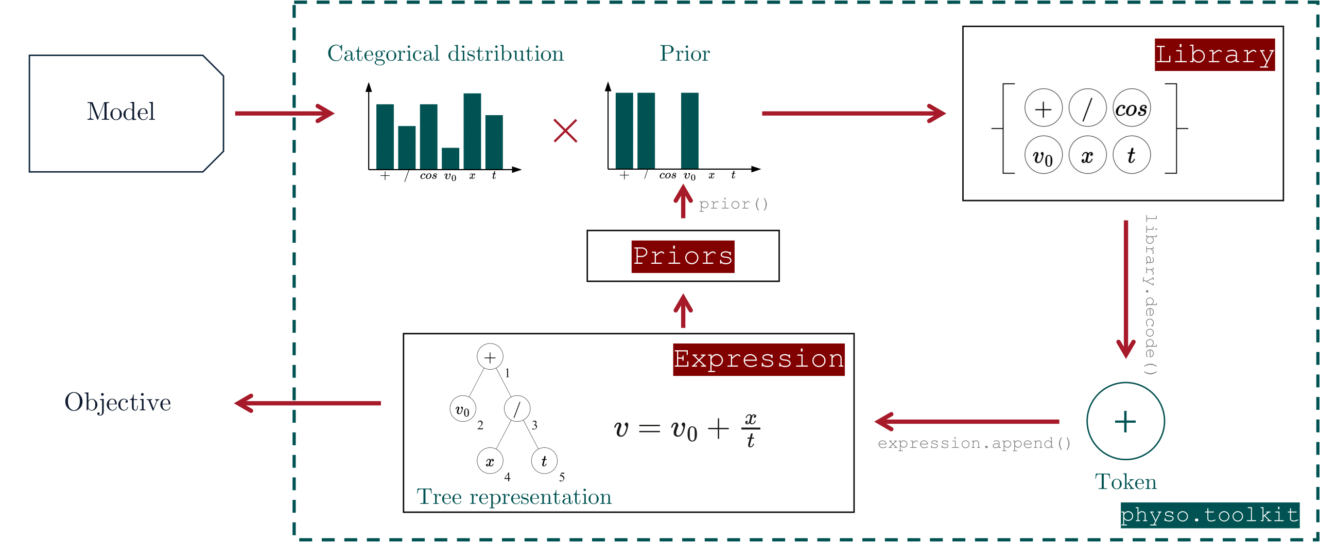
The user’s model produces probability distributions over tokens, which are modulated by deterministic priors to enforce structural or domain-specific constraints.
Tokens are then sampled from the library according to these distributions and appended to the current expression.
The resulting expression can be evaluated for various properties - either formal or based on numerical predictions - to define arbitrary objectives that serve as feedback for the generative process.
Expression manipulation
Refer to this section you wish to learn more about how to manipulate physo expressions (even outside of SR tasks).
Features include:
📦 Flexible export: Expressions can be exported to various formats including (differentiable) python functions, SymPy objects, LaTeX, strings and saved on disk.
⚡️ Evaluation and parameter fitting: Expressions can be numerically evaluated, and their free parameters optimized as needed (in parallel across a batch of equations if desired). Uncertainty can also be taken into account via weights.
🔢 Encoding: Expressions’ numerical encoding can be accessed easily, facilitating the use of expressions for machine learning purposes.
⛓️ Auto-differentiable structures: Expression trees are compatible with automatic differentiation.
🌳 Tree structure navigation: The expression tree can be displayed and navigated. This can be used to access e.g. parent, children, and sibling nodes of any token, and even list their ancestors in a vectorized way across all expressions in the batch.
⚖️ Physical Units information: Physical units of each token is dynamically computed and stored in the expression tree.
📚 One equation, multiple datasets: Expressions can contain dataset-specific free constant values through, allowing for a single equation to be evaluated and fitted across multiple datasets.
Video tutorial (Expressions)
(Coming soon)
Getting started
Reference notebook for this tutorial: 📙demo_expressions.ipynb.
Generating random expressions
physo.toolkit can be used to randomly generate symbolic mathematical equations.
These equations are constructed from a customizable library of tokens-including mathematical operators, variables, and numerical constants-and are encoded in a format suitable for training machine learning models.
Key features include:
📏 Length-controlled sampling: Equations are sampled with a Gaussian prior over expression length.
🏗️ Custom structural priors: You can enforce specific structural properties, such as prohibiting nested trigonometric functions or setting token occurrence constraints.
⚙️ Dimensional analysis: Equations can be generated with physically consistent units, and unit information is preserved throughout the expression tree.
📦 Flexible export: Expressions can be exported to various formats including (differentiable) python functions, SymPy objects, LaTeX, strings and saved on disk.
⚡️ Evaluation and parameter fitting: Expressions can be numerically evaluated, and their free parameters optimized as needed (in parallel across a batch of equations if desired). Uncertainty can also be taken into account via weights.
🔢 Encoding: Expressions’ numerical encoding can be accessed easily, facilitating the use of expressions for machine learning purposes.
⛓️ Auto-differentiable structures: Expression trees are compatible with automatic differentiation.
🌳 Tree structure navigation: The expression tree can be displayed and navigated. This can be used to access e.g. parent, children, and sibling nodes of any token, and even list their ancestors in a vectorized way across all expressions in the batch.
⚖️ Physical Units information: Physical units of each token is dynamically computed and stored in the expression tree.
📚 One equation, multiple datasets: Expressions can contain dataset-specific free constant values through, allowing for a single equation to be evaluated and fitted across multiple datasets.
Video tutorial (Random sampling)
(Coming soon)
Getting started
Reference notebook for this tutorial: 📙demo_random_sampler.ipynb.
A complementary tutorial that shows how to manipulate the symbolic expressions, including inspecting, showing, exporting, evaluating, and more is available in this section of the documentation.
Encoding and decoding expressions
This notebook demonstrates how to numerically encode and decode mathematical expressions using physo.toolkit.
This is useful for any machine learning (ML) tasks that involves symbolic mathematical expressions, such as symbolic regression, equation discovery, or any task that requires the manipulation of mathematical formulas.
Key features include:
🧠 Priors :
physoincludes many deterministic priors that are computed after each token generation that can be used to e.g. bias the search towards certain expressions : this includes length priors, structural priors (e.g. excluding nesting of trigonometric functions such as \(\text{cos}(a+\text{sin}(1/\text{tan}(x)))\)), dimensional analysis priors, prior about the number of occurrences of a token, prior about sub-functions, and more.📦 Flexible export: Expressions can be exported to various formats including (differentiable) python functions, SymPy objects, LaTeX, strings and saved on disk.
⚡️ Evaluation and parameter fitting: Expressions can be numerically evaluated, and their free parameters optimized as needed (in parallel across a batch of equations if desired). Uncertainty can also be taken into account via weights.
🔢 Encoding: Expressions’ numerical encoding can be accessed easily, facilitating the use of expressions for machine learning purposes.
⛓️ Auto-differentiable structures: Expression trees are compatible with automatic differentiation.
🌳 Tree structure navigation: The expression tree can be displayed and navigated. This can be used to access e.g. parent, children, and sibling nodes of any token, and even list their ancestors in a vectorized way across all expressions in the batch.
⚖️ Physical Units information: Physical units of each token is dynamically computed and stored in the expression tree.
📚 One equation, multiple datasets: Expressions can contain dataset-specific free constant values through, allowing for a single equation to be evaluated and fitted across multiple datasets.
Video tutorial (Decoding)
(Coming soon)
Getting started
Reference notebook for this tutorial: 📙demo_encode_decode.ipynb.
A complementary tutorial that shows how to manipulate the symbolic expressions, including inspecting, showing, exporting, evaluating, and more is available in this section of the documentation.
I just want to use physo’s optimization scheme
A tutorial is available for anyone who simply wants to use physo’s free constant optimization scheme - without necessarily diving into symbolic optimization or machine learning.
It contains a simple example of how to optimize constants in a function using PyTorch’s auto-differentiation and LBFGS optimizer.
Notebook: 📙demo_opti_constants.ipynb.